Download LTspice Files
Right-click the link below and decompress the downloaded Archive.zip to extact the LTspice example and plot.def files.
Designers of complex systems need to understand how systems’ components work and how they interact. Design-oriented analysis focuses on analyzing circuits efficiently to promote understanding of how the circuits work. In design-oriented analysis, a complex system is analyzed through a series of idealized and simplified analyses, whose results are combined to represent the system in terms of the interactions of its parts. This is usually a very efficient way to complete the analysis and also provides a conceptual framework for understanding the system’s behavior.
This approach works well for analyzing feedback circuits. The circuit is analyzed with the gain of some amplifier, modelled as a controlled voltage or current source, treated as a variable. System performance is evaluated with the value of the controlled-source gain first set to zero, then to infinity, and finally to arbitrary values. Ultimately the performance of the overall system (input to output gains, input and output impedances, etc.) can be expressed as functions of the feedback loop gain, which depends on the gain of the controlled source. Bode or Nyquist plots of the loop gain can be used to analyze the system’s stability. As we’ll see, this method must be modified if multiple feedback loops affect stability.
The following procedure can be used to find loop gain in circuits with a single feedback loop in manual analysis. The circuit is represented by its linearized equivalent circuit, with independent sources killed. The feedback loop is broken in any branch of the circuit through which all of the feedback flows. The impedance Zin looking into the input side of the feedback loop is found with the output short-circuited. The loop gain T is the small-signal voltage gain found with the output port terminated with Zin. The same value for the loop gain can be found by breaking any branch along the feedback path.
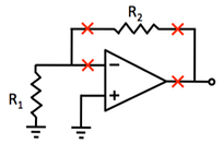
a. Feedback circuit with input sources off and possible breakpoints identified.
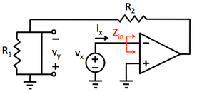
b. Circuit for finding Zin. The vy port is shorted.
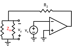
c. Circuit with Zin copied at vy port.
Fig. 1. Finding loop gain in hand analysis. Loop gain is T = vy/vx.
This method for finding loop gain cannot be used directly in SPICE, because breaking the feedback loop changes the operating point, and the loading effects modeled by Zin in hand analysis are not accounted for. Middlebrook [1] showed how these problems can be avoided using a pair of ac simulations, with the circuit excited first with a voltage source and then with a current source. The results of these simulations can then be combined to find the loop gain.
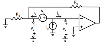
Fig. 2. Middlebrook’s method
for finding loop gain in circuit simulation.
Vz and Iz are applied
one at a time.
Middlebrook’s approach accounts for loading and preserves the dc operating point. However, it works only if the signal flow is unidirectional and the test sources are oriented in the correct direction. An alternate approach proposed by Tian, Kundert et al, [2] removes those limitations, accounting for feedback signal flow in both directions. Tian and Kundert’s approach is implemented as the .stb analysis in Spectre and related Cadence simulators. Wiedmann [3] adapted Tian’s method (as well as several variations on Middlebrook’s method) for use in LTspice. A demonstration of the method is distributed with LTspice as the example circuit LoopGain2.asc. Bode or Nyquist plots of the loop gain found by these methods can be used to analyze stability, including phase margin, gain margin, etc.
Multiple-Loop Feedback
The above approach can correctly analyze stability only in single-loop feedback circuits. If feedback does not all flow through a single circuit branch, a more general technique is needed. In the general technique (Bode [4], Mason [5]), the feedback loops are broken in succession until all feedback is killed. First, a single-loop method is used to find the loop gain T1 through a first controlled source. Next, that controlled source’s gain is killed (set to zero), so that the first feedback loop can be said to be broken. Now, a second loop gain is found by breaking a second circuit branch with the first controlled source gain still set to zero (first feedback loop broken). Let’s call the loop gain of the second loop T21, where the superscript indicates that feedback through loop 1 has been killed. Next, loops 1 and 2 are both killed, and a third loop’s gain, call it T31,2, is found. This procedure, with the loops broken in succession, is repeated until no feedback loops remain.
Factors of the form (1 +Ti) are called loop differences. Factors of the form (1+Ti1,2, ... , i-1), with some feedback loops broken, are called partial loop differences. The product of all of the partial loop differences is the determinant ∆ of the matrix of the circuit’s equations. For a circuit with n feedback loops,
This result is equivalent to the sum-of-products form that can be found from the circuit’s signal-flow graph using Mason’s Gain expression [6].
The feedback loops can be broken in any order, so in the case of a two-loop circuit, the determinant is
The roots of 1 + T(s) = 0 are the circuit’s poles, and if any of the poles have positive real parts the circuit is unstable. Nyquist or Bode plots of T(s) or of the individual loop gains can be used to analyze stability.
Now, if stability is evaluated without accounting for all feedback loops, the missing loop difference factors might have roots with positive real parts, indicating undetected instability. However, if these loops are in fact stable, the additional analysis can be safely skipped. For example, an operational amplifier might be known or assumed to be stable, in which case any internal feedback loops it contains may be safely ignored. Notice also that purely passive circuits, even though they can be represented using controlled sources with feedback, need not be tested for instability, as instability requires gain greater than unity.
Two-Loop Analysis in LTspice
Doing such multiple-loop analysis by hand can be tedious, but in principle it is straightforward. However, there has not until now been a way to do the analysis in circuit simulation. The technique presented here allows analysis of two-loop circuits. The new approach extends Wiedmann’s approach in LTspice, using a pair of probes to break two loops. The results allow all of the factors in Eqn. 2 to be plotted vs. frequency. There are no restrictions on the impedances looking clockwise or counterclockwise from the probes. As in Tian’s approach, the probes can be oriented either way with respect to the direction of signal flow. However, signal flow through the probes must be unidirectional.
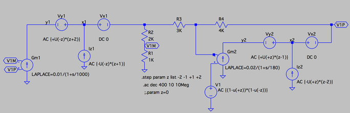
To use the method in LTspice, test probes are placed in series with two circuit branches in the schematic, placed to break all active feedback loops. The test sources have dc values of zero and so do not affect the circuit’s operating point. A parameter z is stepped through the values {-2 -1 +1 +2} in a series of four .AC frequency sweeps. The test sources are controlled by unit step and polynomial functions of z so that the AC value of one source at a time is set to 1.0, while the other test sources are left at zero. No other AC sources should be non-zero during these tests.
Post-processing is done using the “Waveform Viewer” of LTspice, using functions defined in a plot.defs file. These definitions must be included in the user’s plot.defs file. The user must ensure that variables defined in the plot.def don’t conflict with other function definitions. Node names x1, y1, x2 and y2 and the sources Vx1, Vy1, Vx2 and Vy2 used in the probes as ammeters must be correctly included in the schematic.
Note that each function defined in the plot.defs file must be placed on a separate line, with no carriage returns or line feeds.
Functions T1() and T2() as defined in the plot.defs file are the loops gains of each loop with the other loop unaffected, as found using Tian’s method combining voltage and current loop gains. T2P() is the loop gain of Loop 2 with Loop 1 killed and T1P() is the loop gain of Loop 1 with Loop 2 killed. TMason() is the overall loop gain from Eqn. 2.
Example Analysis
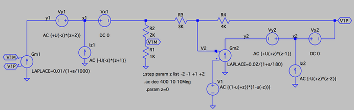
Consider the circuit in Fig. 3, which can be broken in two places to properly determine stability. At first, let’s consider only the DC behavior. The amplifiers are modeled as ideal voltage-controlled current sources, with zero input and output admittances. There is negative feedback around each op amp, and a global loop that includes one inverting and one non-inverting amp, so all loops have negative feedback. Notice that a local feedback signal flows clockwise through R4, while the global feedback through R4 flows counterclockwise.
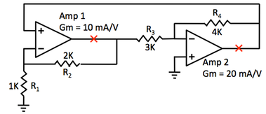
a. Circuit with breakpoints that kill both local feedback loops and a global loop.
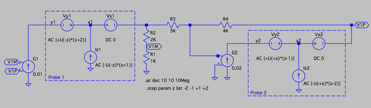
b. LTspice schematic.
Fig. 3. Example circuit with multiple feedback loops.
Let T1 be the loop gain found by probing the signal path at the left-hand amplifier’s output, without disrupting the right-hand loop. The probe simultaneously detects both the left-hand local feedback and the global feedback through and around Amp 2. LTspice’s result for T1() agrees with hand analysis, yielding
![]()
The positive value indicates that the feedback is negative.
The simulated value for T2P() with Loop 2 broken at Amp 2’s output is 120, which is consistent with manual analysis of feedback through Loop 2 with Gm1 set to zero:
These results are useful, but not especially surprising. The positive values of the two loop gains are consistent with negative feedback, and with appropriate compensation the circuit can be stable.
What happens if Loop 2 is broken first? LTspice gives T2() = -164.2. This is consistent with hand analysis, which gives
![]()
The corresponding gain for Loop 1 with Gm2 set to zero is T12 = -Gm1R2 = -20. Both values are negative, because the positive feedback through the non-inverting left-hand amp and through R4 is greater than the negative local feedback around amplifier 2.
The positive feedback in these loops may be surprising, since positive DC feedback with |T| >1 would automatically imply instability in single-loop feedback circuits. As this example shows, positive feedback can be entirely benign in multiple feedback circuits, illustrating why the multiple-loop analysis is necessary.
DC Operating Point Stability
An operating point is a set of DC voltages and currents that satisfies all of a circuit’s large-signal equations. A circuit can have more than one DC operating point. Operating points can classified as either unstable or “potentially stable”. At an unstable operating point, the circuit cannot be compensated: there is no combination of inductors or capacitors that could be added to the circuit to stabilize it by ensuring that all of the circuit’s poles have negative real parts.
Any circuit with an unstable operating point also has at least two additional potentially stable operating points [7]. A circuit intended to work at one operating point may end up in an unintended third condition instead. The existence of an unstable operating point implies that multiple operating points exist.
If a circuit’s determinant is negative at DC, then the corresponding DC operating point is unstable [8]. On the other hand, a positive determinant does not ensure potential stability. A trivial example is a circuit with two uncoupled unstable positive feedback loops. Its determinant would be positive but would factor into the product of two negative loop differences. The sign of the determinant in that case would not depend on the order in which the loop differences are found.
The situation in our example is different. If Loop 2 is broken first, the determinant factors into a product of two negative loop differences. However, if Loop 1 is broken first, the determinant factors into a product of two positive loop differences, and the circuit is potentially stable.
This illustrates the general rule that an operating point is potentially stable if it is possible to factor the determinant using all positive partial loop differences [9].
Compensation
The signs of the factors may depend on the order in which loop gains are reduced to zero, which suggests a “recipe” for compensating the circuit using dominant pole compensation [10]. In the example, the gain of Loop 1 must be reduced to unity before too much phase delay accumulates due to the positive feedback in Loop 2.
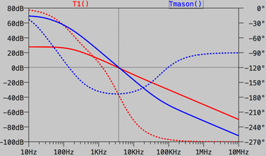
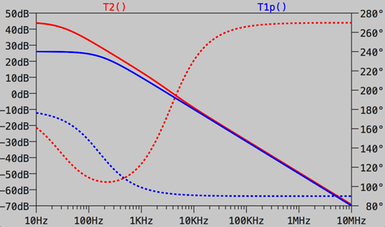
This is demonstrated by the LTspice AC results of the example circuit, with each amplifier simulated with a single pole in its transconductance. In a first simulation, as shown in Fig. 4, both amplifiers have poles at 1 kr/s. Bode plots of T2 and T1p do not reveal much about stability, as the feedback is positive even at DC.
Plots of T1 and of Tmason, however, show that the overall circuit is stable, as T1 and Tmason drop below unity gain with plenty of phase margin.
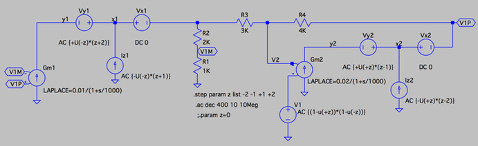
a. LTspice schematic.
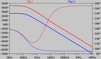
b. Bode plots with Loop 2 broken first.
c. Bode plots of T1 and overall loop gain.
Fig. 4. Circuit of Fig. 3 analyzed in LTspice with feedback broken in two places and with both amplifiers having a pole at 1000 r/s.
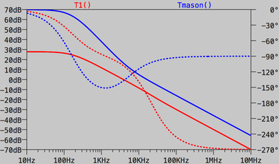
If Amp 2’s pole is set to a much lower frequency than Amp 1’s, the phase margin is greatly reduced. In a second set of simulations, as shown in Fig. 5, Amp 2’s pole is lowered to 180 r/s while Amp 1’s pole is left at 1 kr/s. Again, Bode plots with loop 2 broken first are ambiguous. However, plots of T1 and Tmason both show a phase margin of about 7 degrees, with unity-gain frequency near 3.6 kHz.
a. LTspice schematic.
b. Bode plots with Loop 2 broken first.
c. Bode plots of T1 and overall loop gain.
Fig. 5. Circuit of Fig. 3 analyzed with the Amp 2’s pole reduced to 180 r/s. The phase margin is only about 7 degrees.
In Fig. 6, the closed-loop gain of the circuit from Fig. 4 is plotted by commenting out the .step command and setting parameter z to zero to disable the probe sources. A single input source is given a non-zero value as shown in the figure.
a. LTspice schematic.
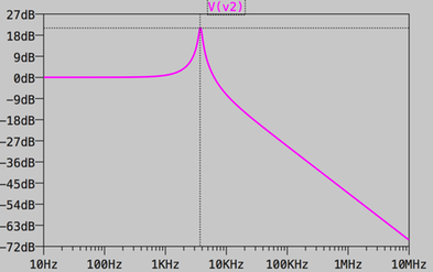
b. Closed-loop gain.
Fig. 6. Closed-loop analysis of the circuit from Fig. 5.
The resulting closed-loop response has a strong peak near the unity-gain frequency of Tmason. The two-loop analysis shows that effects of both loops must be considered and that feedback loop 1 must have the dominant pole.
Limitations
The two-loop analysis presented here gives proper results only when the test probes are placed to detect all active feedback. The example circuit could have been probed at the Amp 2’s input rather than the output, and the direction of the probes could be swapped without changing the results. But the method doesn’t work if significant feedback flows in both directions through a probe. For example, it may seem that Probe 2 could be placed in series with R4. However, Loop 2’s feedback flows right to left through R4 while Loop 1’s feedback flows left to right. The two-loop algorithm does not break both paths simultaneously, and the algorithm does not give meaninful results when used that way.
How the Two-Loop Algorithm Works
[Note: More details about the implementation will be provided at a later time.]
To understand how the two-loop algorithm works, it helps to first review Wiedmann’s implementation for single-loop loop gains [11]. Separately applying a shunt current probe source and then a series voltage source leads to a pair of equations for the voltages and currents at the x and y ports on either side of the probes. These equations can be solved using using Cramer’s Rule to find the voltage and current gains between the x and y ports under conditions equivalent to Middlebrook’s multiple-input null conditions. In principle one could find the ratio of the two sources needed to achieve various null conditions, and then find the forward and reverse voltage and current gains with those conditions met. In practice, we don’t need to explicitly solve for the conditions and can get the gains directly. The gains are then combined to get the final results. Wiedmann’s single-loop case is based on solution of four 2x2 determinants, although the final result for loop gains reduces to fairly simple expressions involving just one 2x2 determinant.
Extending the algorithm to two loops requires applying Cramer’s Rule to 4x4 matrices. Applying the null conditions requires finding four 3x3 and four 2x2 determinants, equivalent to a series of triple-input double-null analyses. The results are combined to find the gains in one loop with the gain through the other loop killed. To allow each pair of probes to be placed in either direction with respect to feedback signal flow, the determinants are found for each of four different matrices. With the possibility of forward or reverse gains requiring both current and voltage gains, there are a lot of possibilities to account for. Ultimately all of the results are combined using a formula that gives the same result for all probe orientations.
It’s possible that there is a simpler way to do these calculations that I haven’t found. Extending the analysis to allow for a third feedback loop would require finding determinants of 6x6 matrices. The algebraic complexity of finding the determinant of an nxn matrix grows as n!, so directly extending the method will be quite complicated. Some approach using symbolic recursion seems like the most promising. If someone figures out how to do it, I hope they’ll let me know.
[UPDATE: I was contacted by Jochen Verbrugghe of the Intec Design group of the faculty of Engineering and Architecture of Ghent University. He and his colleagues have implemented Middlebrook’s General Feedback Theorem in Cadence’s design system ([12], [13]). He reports that his approach yields the correct results for my examples, and believes his approach is applicable for systems with more than two loops. We haven’t yet had a chance to work through the details. His results appear very promising.]
References
[1] R. D. Middlebrook, “Measurement of Loop Gain in Feedback Systems”, International Journal of Electronics, vol. 38, no. 4, pp. 485-512, April 1975.
[2] Tian, et al., “Striving for Small-Signal Stability”, IEEE Circuits and Devices Magazine, vol. 17, no. 1, pp. 31-41, January 2001.
[3] F. Wiedmann, “Loop Gain Simulation”.
[4] H. W. Bode, Network Analysis and Feedback Amplifier Design, Van Nostrand, New York, 1945. pp. 157.
[5] S. J. Mason, “Feedback Theory -- Some properties of signal flow graphs,” Proceedings of the IRE, vol. 41, pp. 1144-1156, September, 1953.
[6] S. J. Mason, "Feedback theory-further properties of signal flow graphs," Proceedings of the IRE, vol. 44, pp. 920-926, July, 1956.
[7] M. M. Green, A. N. Willson, “(Almost) half of all operating points are unstable,” IEEE Transactions on Circuits and Systems – Part I, vol. 41, pp. 286-293, April 1994.
[8] M. M. Green, A. N. Willson, “How to identify unstable dc operating points,” IEEE Transactions on Circuits and Systems – Part I, vol. 39, pp. 840-844, Oct. 1992.
[9] M. E. Fisher, A.T. Fuller, “On the stabilization of matrices and the convergence of linear iterative processes,” Proc. Cambridge Philos. Soc., 54 (1958), pp. 417–425.
[10] C.S. Ballantine “Stabilization by a diagonal matrix,” Proc. Amer. Math. Soc., 25 (1970), pp. 729–734.
[11] A. Petrini, “Loop gain calculation with Spice”.
[12] J. Verbrugghe, B. Moeneclaey and J. Bauwelinck, "Implementation of the dissection theorem in cadence virtuoso", International Conference on Synthesis, Modeling, Analysis and Simulation Methods and Applications to Circuit Design (SMACD), September 19-21, 2012, Seville, Spain, pp. 145 - 148.
[13] J. Verbrugghe, B. Moeneclaey and J. Bauwelinck, "Integration of the general network theorem in ADE and ADE XL: toward a deeper insight into circuit behavior", CDNLive, Cadence User Conference, EMEA-Munich, Germany, May 19-21, 2014, paper AC12, Nr. AC12, May 19-21, 2014, Munich, Germany.
Appendix: Plot.Defs file for Multiple-Loop Feedback Analysis
* File:
/Users/rob/Documents/LTspice/plot.defs
* These function definitions must be included
in your plot.defs file. Make sure they
* do not conflict with other definitions.
Make sure nodes x1,y2,x2 and y2 are defined and
* connected properly in your circuit.
*
* Be sure every function definition appears
as a separate line.
*
* T1() and T2() are the loop gains as would
be found using the LoopGain2 (Tian) method.
* T1p() is the gain of loop1 when loop2’s
feedback is killed.
* T2p() is the gain of loop2 when loop1’s
feedback is killed.
* A Bode plot Tmason() can be used to
determine stability of the overall circuit.
* Breaking loops 1 and 2 must kill all active
feedback.
.func dT1()=-I(vy1)@1*V(y1)@2+I(vy1)@2*V(y1)@1
.func dT2()=-I(vy2)@3*V(y2)@4+I(vy2)@4*V(y2)@3
.func T1() = 1/(I(vy1)@1-V(y1)@2 -2*dT1())-1
.func T2() = 1/(I(vy2)@3-V(y2)@4 -2*dT2())-1
.func
dxy11()=-v(x1)@2*i(vy2)@3*v(y2)@4-v(x1)@3*i(vy2)@4*v(y2)@2-v(x1)@4*i(vy2)@2*v(y2)@3+v(x1)@4*i(vy2)@3*v(y2)@2+v(x1)@2*i(vy2)@4*v(y2)@3+v(x1)@3*i(vy2)@2*v(y2)@4
.func
dxy22()=-i(vx1)@1*i(vy2)@3*v(y2)@4-i(vx1)@3*i(vy2)@4*v(y2)@1-i(vx1)@4*i(vy2)@1*v(y2)@3+i(vx1)@4*i(vy2)@3*v(y2)@1+i(vx1)@1*i(vy2)@4*v(y2)@3+i(vx1)@3*i(vy2)@1*v(y2)@4
.func dxy33()=-i(vx1)@1*v(x1)@2*v(y2)@4+v(y2)@1*v(x1)@2*i(vx1)@4-i(vx1)@2*v(x1)@4*v(y2)@1+v(y2)@2*v(x1)@4*i(vx1)@1-i(vx1)@4*v(x1)@1*v(y2)@2+v(y2)@4*v(x1)@1*i(vx1)@2
.func
dxy44()=i(vx1)@1*v(x1)@2*i(vy2)@3-i(vy2)@1*v(x1)@2*i(vx1)@3+i(vx1)@2*v(x1)@3*i(vy2)@1-i(vy2)@2*v(x1)@3*i(vx1)@1+i(vx1)@3*v(x1)@1*i(vy2)@2-i(vy2)@3*v(x1)@1*i(vx1)@2
.func dxy1133()={-v(x1)@2*v(y2)@4+v(x1)@4*v(y2)@2}
.func
dxy1144()={+v(x1)@2*i(vy2)@3-v(x1)@3*i(vy2)@2}
.func
dxy2233()={-i(vx1)@1*v(y2)@4+i(vx1)@4*v(y2)@1}
.func dxy2244()={+i(vx1)@1*i(vy2)@3-i(vx1)@3*i(vy2)@1}
.func
dyx11()=-v(y1)@2*i(vx2)@3*v(x2)@4-v(y1)@3*i(vx2)@4*v(x2)@2-v(y1)@4*i(vx2)@2*v(x2)@3+v(y1)@4*i(vx2)@3*v(x2)@2+v(y1)@2*i(vx2)@4*v(x2)@3+v(y1)@3*i(vx2)@2*v(x2)@4
.func dyx22()=
I(vy1)@1*I(vx2)@3*V(x2)@4+I(vy1)@3*I(vx2)@4*V(x2)@1+I(vy1)@4*I(vx2)@1*V(x2)@3-I(vy1)@4*I(vx2)@3*V(x2)@1-I(vy1)@1*I(vx2)@4*V(x2)@3-
I(vy1)@3*I(vx2)@1*V(x2)@4
.func
dyx33()=-i(vy1)@1*v(y1)@2*v(x2)@4+v(x2)@1*v(y1)@2*i(vy1)@4-i(vy1)@2*v(y1)@4*v(x2)@1+v(x2)@2*v(y1)@4*i(vy1)@1-i(vy1)@4*v(y1)@1*v(x2)@2+v(x2)@4*v(y1)@1*i(vy1)@2
.func
dyx44()=-i(vy1)@1*v(y1)@2*i(vx2)@3+i(vx2)@1*v(y1)@2*i(vy1)@3-i(vy1)@2*v(y1)@3*i(vx2)@1+i(vx2)@2*v(y1)@3*i(vy1)@1-i(vy1)@3*v(y1)@1*i(vx2)@2+i(vx2)@3*v(y1)@1*i(vy1)@2
.func dyx1133()={-v(y1)@2*v(x2)@4+v(y1)@4*v(x2)@2}
.func dyx1144()={-v(y1)@2*I(Vx2)@3+v(y1)@3*I(Vx2)@2}
.func dyx2233()={
I(vy1)@1*v(x2)@4-I(Vy1)@4*v(x2)@1}
.func dyx2244()={
I(vy1)@1*I(vx2)@3-I(vy1)@3*I(vx2)@1}
.func
dxx11()=V(x1)@2*I(vx2)@3*V(x2)@4+V(x1)@3*I(vx2)@4*V(x2)@2+V(x1)@4*I(vx2)@2*V(x2)@3-V(x1)@4*I(vx2)@3*V(x2)@2-V(x1)@2*I(vx2)@4*V(x2)@3-V(x1)@3*I(vx2)@2*V(x2)@4
.func
dxx22()=I(vx1)@1*I(vx2)@3*V(x2)@4+I(vx1)@3*I(vx2)@4*V(x2)@1+I(vx1)@4*I(vx2)@1*V(x2)@3-I(vx1)@4*I(vx2)@3*V(x2)@1-I(vx1)@1*I(vx2)@4*V(x2)@3-I(vx1)@3*I(vx2)@1*V(x2)@4
.func dxx33()=i(vx1)@1*v(x1)@2*v(x2)@4-v(x2)@1*v(x1)@2*i(vx1)@4+i(vx1)@2*v(x1)@4*v(x2)@1-v(x2)@2*v(x1)@4*i(vx1)@1+i(vx1)@4*v(x1)@1*v(x2)@2-v(x2)@4*v(x1)@1*i(vx1)@2
.func
dxx44()=i(vx1)@1*v(x1)@2*i(vx2)@3-i(vx2)@1*v(x1)@2*i(vx1)@3+i(vx1)@2*v(x1)@3*i(vx2)@1-i(vx2)@2*v(x1)@3*i(vx1)@1+i(vx1)@3*v(x1)@1*i(vx2)@2-i(vx2)@3*v(x1)@1*i(vx1)@2
.func dxx1133()={v(x1)@2*v(x2)@4-v(x1)@4*v(x2)@2}
.func
dxx1144()={+v(x1)@2*i(vx2)@3-v(x1)@3*i(vx2)@2}
.func
dxx2233()={+i(vx1)@1*v(x2)@4-i(vx1)@4*v(x2)@1}
.func
dxx2244()={+i(vx1)@1*i(vx2)@3-i(vx1)@3*i(vx2)@1}
.func dyy11()=
V(y1)@2*I(vy2)@3*V(y2)@4+V(y1)@3*I(vy2)@4*V(y2)@2+V(y1)@4*I(vy2)@2*V(y2)@3-V(y1)@4*I(vy2)@3*V(y2)@2-V(y1)@2*I(vy2)@4*V(y2)@3-V(y1)@3*I(vy2)@2*V(y2)@4
.func
dyy22()=-I(vy1)@1*I(vy2)@3*V(y2)@4-I(vy1)@3*I(vy2)@4*V(y2)@1-I(vy1)@4*I(vy2)@1*V(y2)@3+I(vy1)@4*I(vy2)@3*V(y2)@1+I(vy1)@1*I(vy2)@4*V(y2)@3+I(vy1)@3*I(vy2)@1*V(y2)@4
.func
dyy33()=+i(vy1)@1*v(y1)@2*v(y2)@4-v(y2)@1*v(y1)@2*i(vy1)@4+i(vy1)@2*v(y1)@4*v(y2)@1-v(y2)@2*v(y1)@4*i(vy1)@1+i(vy1)@4*v(y1)@1*v(y2)@2-v(y2)@4*v(y1)@1*i(vy1)@2
.func dyy44()=-i(vy1)@1*v(y1)@2*i(vy2)@3+i(vy2)@1*v(y1)@2*i(vy1)@3-i(vy1)@2*v(y1)@3*i(vy2)@1+i(vy2)@2*v(y1)@3*i(vy1)@1-i(vy1)@3*v(y1)@1*i(vy2)@2+i(vy2)@3*v(y1)@1*i(vy1)@2
.func dyy1133()={+v(y1)@2*v(y2)@4-v(y1)@4*v(y2)@2}
.func
dyy1144()={-v(y1)@2*i(vy2)@3+v(y1)@3*i(vy2)@2}
.func
dyy2233()={-i(vy1)@1*v(y2)@4+i(vy1)@4*v(y2)@1}
.func
dyy2244()={+i(vy1)@1*i(vy2)@3-i(vy1)@3*i(vy2)@1}
.func Sxx()=dxx11()*dxx22()*dxx33()*dxx44()
.func Sxy()=dxy11()*dxy22()*dxy33()*dxy44()
.func Syx()=dyx11()*dyx22()*dyx33()*dyx44()
.func Syy()=dyy11()*dyy22()*dyy33()*dyy44()
.func Kxx()=dxx1133()+dxx1144()+dxx2233()+dxx2244()
.func Kxy()=dxy1133()+dxy1144()+dxy2233()+dxy2244()
.func Kyx()=dyx1133()+dyx1144()+dyx2233()+dyx2244()
.func Kyy()=dyy1133()+dyy1144()+dyy2233()+dyy2244()
.func Qxx2()=dxx11()+dxx22()
.func Qxy2()=dxy11()+dxy22()
.func Qyx2()=dyx11()+dyx22()
.func Qyy2()=dyy11()+dyy22()
.func Qxx1()=dxx33()+dxx44()
.func Qxy1()=dxy33()+dxy44()
.func Qyx1()=dyx33()+dyx44()
.func Qyy1()=dyy33()+dyy44()
.func
FD1()=Syy()*Kyx()+Sxy()*Kxx()+Syx()*Kyy()+Sxx()*Kxy()
.func
FD2()=Syy()*Kxy()+Sxy()*Kyy()+Syx()*Kxx()+Sxx()*Kyx()
.func
FN1()=Syy()*Qyx1()+Sxy()*Qxx1()+Syx()*Qyy1()+Sxx()*Qxy1()
.func FN2()=Syy()*Qxy2()+Sxy()*Qyy2()+Syx()*Qxx2()+Sxx()*Qyx2()
.func T1p()=1/(FD1()/FN1()-2)
.func T2p()=1/(FD2()/FN2()-2)
.func TMason()={T1()+T2P()+T1()*T2P()}